RL-LAB TERMINAL // ERCOT_QLEARNING_V12
Teaching an RL Agent to Bid in a Realistic Electricity Market
A data-driven, multi-agent Q-learning thesis on how power generators can bid strategically when the market refuses to sit still.
Research Log
- [x]Environment built
- [x]Historical data ingested
- [x]Baseline policies
- [x]Reward function redesigned
- [x]Multi-agent support
- [ ]DQN
- [ ]PPO
The Problem: Selling Power Is Not as Simple as "Charge More"
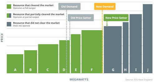
Wholesale electricity markets are basically large, fast, slightly terrifying auctions. Every day, generators submit bids describing how much electricity they are willing to sell and at what price. The market then sorts those bids from cheapest to most expensive, clears enough supply to meet demand, and determines who gets dispatched.
The awkward part is that generators must submit those bids before they know exactly what demand, renewable output, competitor behaviour, or clearing prices will look like. Bid too aggressively and you might earn a great margin. Bid too aggressively at the wrong time and you may sell exactly zero electricity, which is less fun.
My thesis asks a practical question: can a reinforcement-learning agent learn when to bid competitively, when to hold margin, and how to balance the two better than a fixed rule-based strategy?
The Project
For my undergraduate thesis, I built a reinforcement-learning framework for strategic bidding in day-ahead electricity markets. The system uses historical ERCOT market data, including demand, locational marginal prices, fuel mix information, and demand forecasts, to create a simulated environment where generators can repeatedly submit bids and learn from the consequences.
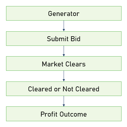
Each training episode represents a 24-hour operating day. At every hour, the agent observes the market context, chooses a bid price and quantity, clears against a simulated supply stack, receives a profit-based reward, and updates its estimate of which decisions were worth making.
The goal was not to build a magic money printer for the electrical grid. It was to build a transparent and reproducible framework for studying how strategic bidding policies emerge when demand, cost, competition, and uncertainty all matter at the same time.
Turning a Messy Market Into Something an Agent Can Learn From
Real electricity markets are not clean textbook environments. Generators do not know every competitor's cost curve. Demand forecasts are imperfect. Renewable output moves around. Market participants can influence one another. In other words: it is much closer to a partially observable game than a neat little spreadsheet.
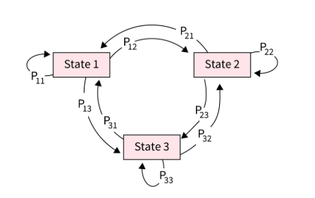
To make the problem tractable, we modelled the market as a finite Markov Decision Process. The state captures the information a generator could reasonably use when bidding, including recent price and load history, a rolling demand forecast, and time-of-day features.
The action is a discrete price-and-quantity bid. The reward is realized profit after market clearing, with constraints and penalties to discourage infeasible or excessively risky bids. This lets the agent learn from experience rather than assuming we know the exact market dynamics in advance, which, thankfully, is useful because we very much do not.
What the Agent Actually Sees and Does
The model uses tabular Q-learning: instead of hiding everything inside a black-box neural network, the agent maintains an explicit value estimate for each discretized state-action pair. That makes the learned policy inspectable, debuggable, and much easier to challenge when it does something questionable.
- State: recent demand and price behaviour, forecast demand, and time features
- Action: a discrete bid price and bid quantity
- Reward: realized profit after clearing, adjusted for feasibility and risk controls
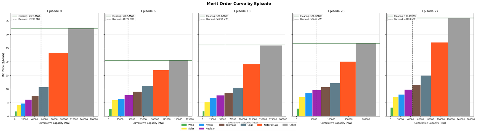
- Market logic: uniform-price clearing, partial clearing, merit-order dispatch, and simulated competitors
- Learning: Q-learning with softmax exploration and decaying learning dynamics
- Competition: single-agent, three-agent, and five-agent market scenarios
I also used warm starts based on economically sensible cost-plus policies. Starting from a reasonable baseline gave the agents a better first guess than trying random things until the grid loses patience.
| Parameter Name | Type | What it controls | 1-Agent | 3-Agent | 5-Agent |
|---|---|---|---|---|---|
| brgap k eval | Threshold | How often the bid-reward gap is evaluated for convergence checks. | 60 | 60 | 60 |
| brgap late save threshold | Threshold | Minimum late-training improvement needed before saving a policy. | 0.10 | 0.25 | 0.25 |
| brgap train mode | Threshold | Policy used when the bid-reward gap routine continues training. | greedy q | greedy q | greedy q |
| late save min episodes | Threshold | Earliest episode where late-training save logic can activate. | 1500 | 1750 | 1750 |
| q delta threshold | Threshold | Q-value movement threshold used to judge whether learning has stabilized. | 0.2 | 0.2 | 0.2 |
| q delta window | Threshold | Number of recent Q-delta measurements used for stabilization checks. | 10 | 10 | 10 |
| risk penalty lambda | Risk | Strength of the penalty applied to riskier bidding behaviour. | 0.0 | 0.0 | 0.0 |
| max notional q | Risk | Upper bound on the notional bid quantity exposed to the policy. | 0.95 | 0.95 | 0.95 |
| warm start q | Learning | Whether the Q-table starts from an economically sensible baseline. | True | True | True |
| policy freeze k | Learning | How long a learned policy is held fixed before updating again. | 5 | 10 | 10 |
| learning rate | Learning | Initial size of each Q-learning update. | 1.0 | 1.0 | 1.0 |
| learning rate exponent | Learning | Controls how quickly learning-rate effects decay over training. | 0.7 | 0.7 | 0.7 |
| temperature | Temperature | Initial softness of the action-selection distribution. | 1.0 | 1.0 | 1.0 |
| temperature decay | Temperature | Rate at which exploration cools as training progresses. | 0.9993 | 0.9993 | 0.9995* |
| temperature min | Temperature | Lower bound on exploration temperature. | 0.05 | 0.05 | 0.05 |
| temperature mode | Temperature | Schedule used to reduce exploration over time. | exp decay | exp decay | exp decay |
*Slower decay in the 5-agent case sustains exploration over a larger joint action space.
| Model Setting | Value Used | Why it matters |
|---|---|---|
| State representation | Discretized price, load, forecast, and time features | Turns noisy market context into a finite state space the Q-table can learn over. |
| Action representation | Finite bid grid over price and quantity | Keeps bidding decisions transparent and compatible with tabular Q-learning. |
| Reward definition | Profit from cleared quantity, clearing price, and sampled marginal cost | Aligns learning with economic payoff instead of only dispatch frequency. |
| Market clearing | Uniform-price, merit-order clearing with partial clearing at the margin | Captures the supply-stack mechanics that determine whether bids clear. |
| Opponent model | Fuel-band Gaussian bid sampling in multi-agent cases | Creates heterogeneous competitors without needing private plant-level cost curves. |
| Marginal cost proxy | Henry Hub gas price distribution | Grounds generation cost variation in real energy-market data. |
Multi-Agent Competition: Where It Gets Interesting
A single generator learning in isolation is useful, but electricity markets are competitive by design. To move beyond that simplified case, the framework supports multiple RL agents bidding into the same market at the same time.
Each agent maintains its own Q-table and chooses its own bid, while the market clears everyone together. This introduces the inconvenient but realistic fact that one agent's "good strategy" may stop being good once other agents begin adapting too.
That turns the problem into a repeated stochastic game: agents are not only learning the market, they are learning in a market shaped by other learners. That is a much more accurate reflection of competitive environments than assuming every competitor politely remains frozen in place.
Results: Did It Work?
Yes, within the assumptions of the simulator, the learned policies outperformed the simpler benchmark strategies we tested against.
In the single-agent ERCOT evaluation, the RL policy achieved a mean episodic profit 29.2% higher than the best cost-plus-markup baseline. In the five-agent scenario, that performance gap increased to 79.17%.
The important part was not merely that the agent earned more simulated profit. It learned a different kind of strategy: rather than applying the same percentage markup regardless of market conditions, it adapted its bid price and quantity to where it expected to sit in the merit order.
In plain English: it learned that sometimes the best move is not to bid the highest price possible. Sometimes the smart move is to price competitively enough to actually clear. A lesson that applies to more than just electricity markets.
- Compared learned policies against cost-plus-markup and historical-quantile baselines
- Evaluated performance across single-agent, three-agent, and five-agent market settings
- Tracked Q-value stabilization, reward behaviour, and policy convergence diagnostics
- Tested sensitivity to warm starts, exploration schedules, risk controls, demand changes, and competition assumptions
- Examined learned bids for economic plausibility instead of treating raw profit as the only metric that matters
Training Diagnostics
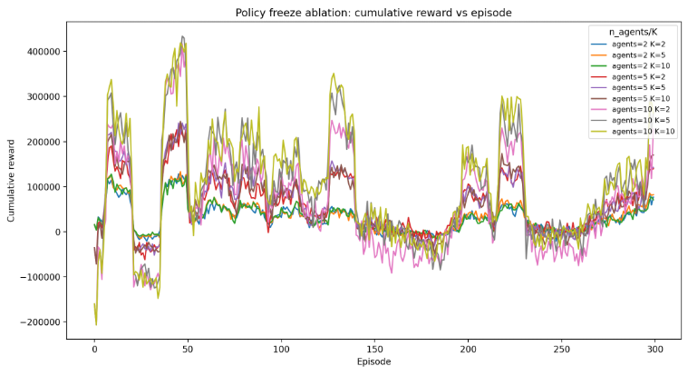
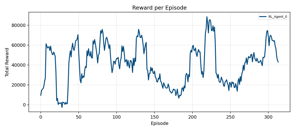
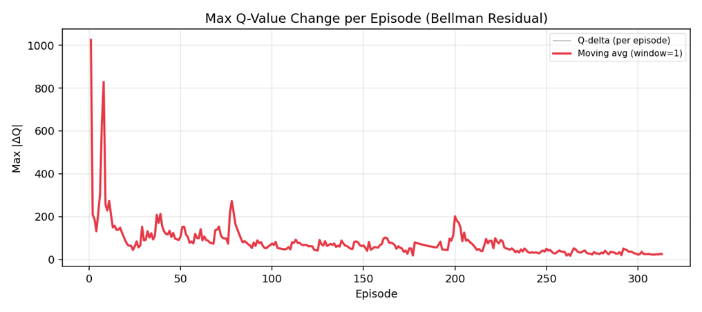
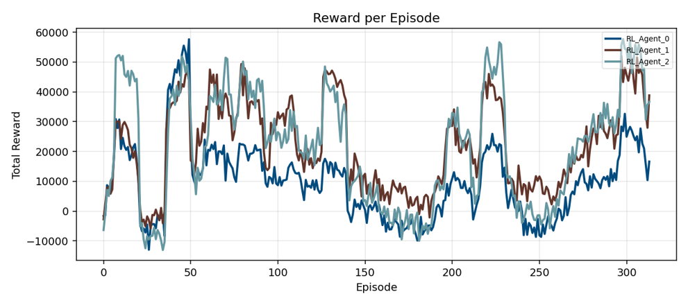
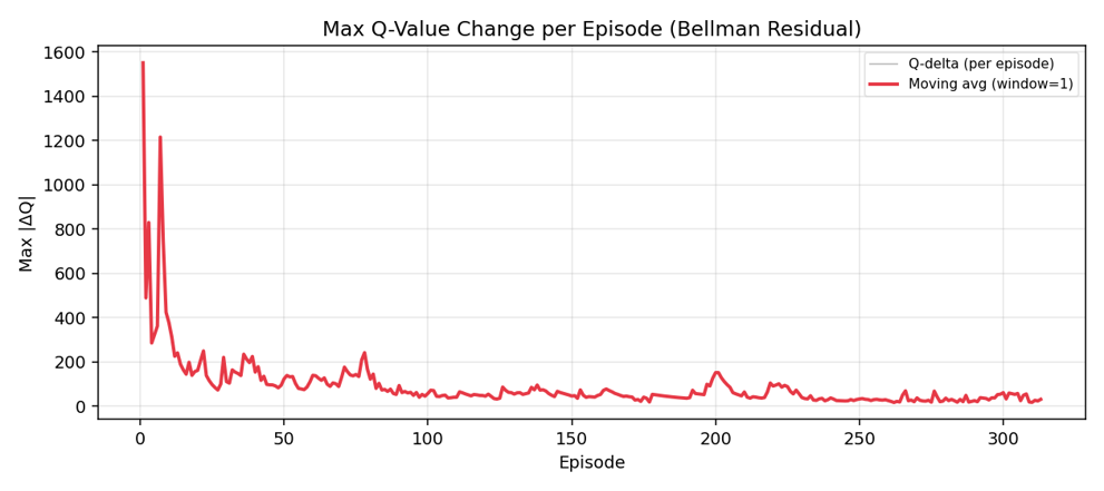
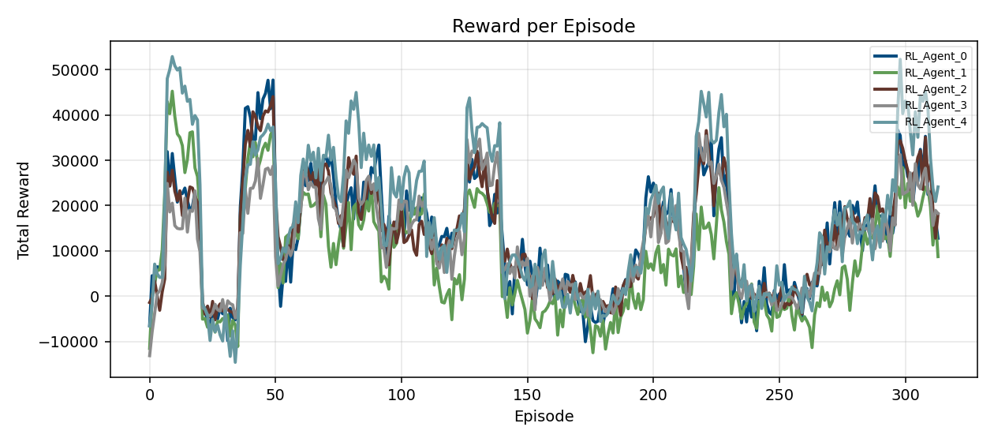
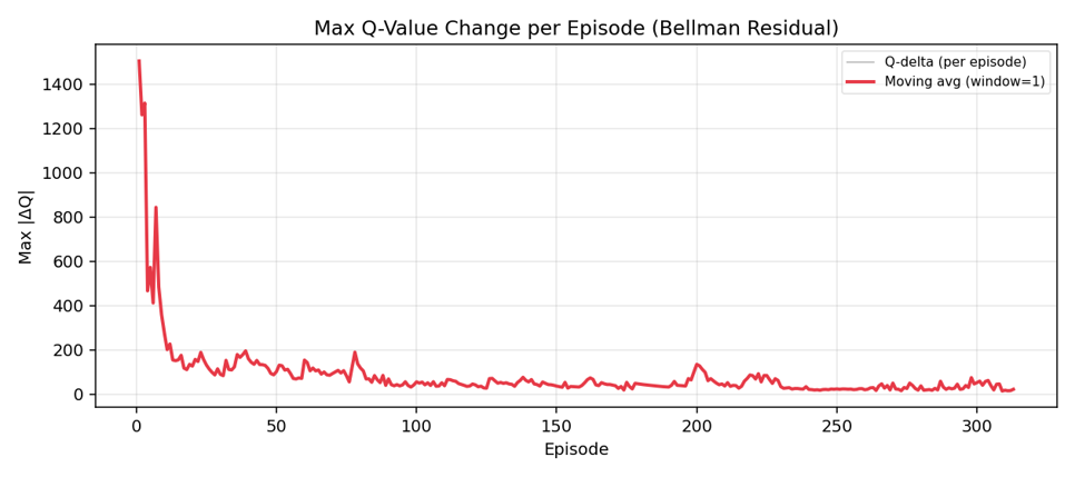
The reward curves show how realized profit evolved during training, while the max Q-value change plots track whether the learned value function was stabilizing. Across the one-, three-, and five-agent settings, the early updates are large and noisy before settling into smaller policy adjustments.
Benchmark Results
The raw benchmark tables compare the learned RL policies against fixed cost-plus bidding rules. The three-agent case is dominated by an undercutting strategy, while the five-agent case shows a more sophisticated policy tracking the marginal resource.
| Policy | Mean Profit ($) | Profit Std ($) | Win Rate (%) | Profit Share (%) | Mean Bid ($/MWh) |
|---|---|---|---|---|---|
| Cost-Plus 25% | 51,086 | 61,127 | 10.71 | 10.45 | 294.55 |
| Cost-Plus 30% | 49,091 | 58,893 | 3.57 | 10.00 | 294.55 |
| Cost-Plus 35% | 45,872 | 53,992 | 3.57 | 9.35 | 294.55 |
| RL Agent 0 | 56,353 | 61,714 | 35.71 | 27.94 | 64.70 |
| RL Agent 1 | 74,392 | 92,194 | 28.57 | 22.60 | 58.52 |
| RL Agent 2 | 66,661 | 86,542 | 17.86 | 19.65 | 63.66 |
| Policy | Mean Profit ($) | Profit Std ($) | Win Rate (%) | Profit Share (%) | Mean Bid ($/MWh) | Min ($) | CVaR10 ($) |
|---|---|---|---|---|---|---|---|
| Cost-Plus 25% | 41,814 | 51,638 | 7.14 | 7.49 | 294.55 | 0.00 | 0.00 |
| Cost-Plus 30% | 44,488 | 50,992 | 0.00 | 7.48 | 294.55 | 0.00 | 0.00 |
| Cost-Plus 35% | 43,664 | 49,461 | 3.57 | 7.40 | 294.55 | 0.00 | 0.00 |
| RL Agent 0 | 54,373 | 68,429 | 17.86 | 15.61 | 63.82 | 2,034 | 3,206 |
| RL Agent 1 | 80,295 | 98,088 | 42.86 | 20.94 | 81.68 | 2,018 | 2,285 |
| RL Agent 2 | 56,320 | 65,311 | 3.57 | 13.43 | 78.75 | 1,380 | 1,930 |
| RL Agent 3 | 63,471 | 91,224 | 0.00 | 13.82 | 79.90 | -2,265 | -159 |
| RL Agent 4 | 71,663 | 108,618 | 25.00 | 13.80 | 60.61 | -806 | 2,092 |
Validation Checks
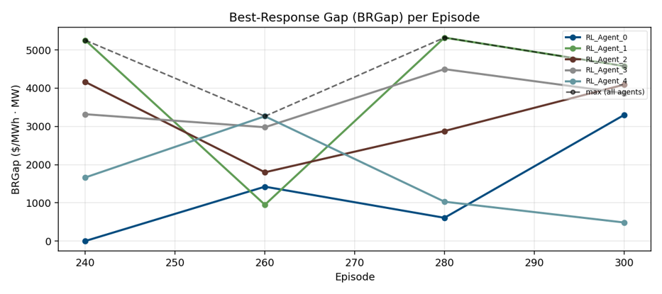
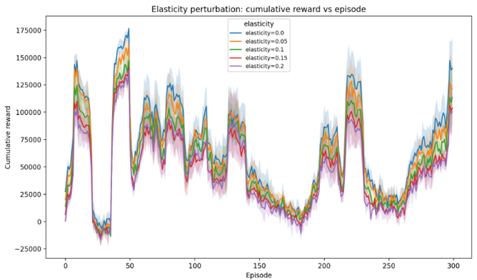
I also checked whether the learned policies behaved sensibly under market-mechanism and robustness diagnostics: best-response gaps, merit-order clearing behaviour, and demand elasticity perturbations.
What I Learned From Building It
The hardest part of this project was not implementing Q-learning. It was deciding what the agent should be allowed to know, what the simulator should approximate, and how to test whether a strong result reflected useful learning instead of an accidental loophole in the environment.
That meant treating model validation as part of the engineering work, not an appendix written after the fun part. I evaluated baseline performance, explored sensitivity to modelling assumptions, monitored convergence behaviour, and documented limitations around discretization, opponent modelling, market constraints, and missing operational details.
The project reinforced something I enjoy about quantitative software work: the code is only useful when the modelling choices behind it are defensible. A clean implementation of the wrong market is still the wrong market.
Want the Technical Version?
The full thesis covers the MDP formulation, simulated market-clearing process, learning algorithm, validation approach, convergence analysis, results, limitations, and future work toward deeper function approximation and more realistic operational constraints.
- GitHub: capstone-optimal-bidding
- Finished Thesis: Read the full paper
- Final Presentation: View the project presentation